Data Visualization Final Paper

By Shreyas Meher

December 7, 2021

Introduction

There has been considerable research done on the ecological impact of the growing consumption patterns all across the world (Toth and Szigeti 2016). The theory follows Malthusian concepts and tenets, wherein the developed world and now the developing nations are increasing their consumption of resources available in the environment for a marginal increase in economic growth and development. Malthus decried the explosive population growth and the strain that it caused on the resources, thus leading to a stagnation in world income and income per capita. Operationalization of the ability of certain countries to recover resources and their rate of exhaustion of resources is another question, and is the focus of the Global Footprint Network (GFN), which is the data-set used for this project.

This project is exploratory in nature, and looks to see how Bio-capacity and Ecological Footprint and the relationship between them and various other variables plays out using the GFN database. The main purpose for this paper lies in the question regarding sustainable development goals and whether consumption patterns around the world are indeed changing. For this, various data visualization methods as gleaned from the class will be used for the purposes of this paper.

knitr::opts_chunk$set(warning = FALSE, message = FALSE) 

footprint <- read.csv("countries.csv")

library(dplyr) # data wrangling
library(tidyr) # data wrangling
library(ggplot2) # plot
library(plotly) # interactive plot
library(ggthemes) # themes for ggplot2
library(extrafont) # fonts for ggplot2
library(RColorBrewer) # colors

Variable definitions

To get us started off, I will mention key definitions that are crucial to understand for this project. The GFN have defined the variables, which is what I am noting down in this section.

Ecological Footprint - A measure of how much area of biologically productive land and water an individual, population, or activity requires to produce all the resources it consumes and to absorb the waste it generates, using prevailing technology and resource management practices. The Ecological Footprint is usually measured in global hectares. Because trade is global, an individual or country’s Footprint includes land or sea from all over the world. Without further specification, Ecological Footprint generally refers to the Ecological Footprint of consumption. Ecological Footprint is often referred to in short form as Footprint.

Biocapacity - The capacity of ecosystems to regenerate what people demand from those surfaces. Life, including human life, competes for space. The biocapacity of a surface represents its ability to renew what people demand. Biocapacity is therefore the ecosystems’ capacity to produce biological materials used by people and to absorb waste material generated by humans, under current management schemes and extraction technologies. Biocapacity can change from year to year due to climate, management, and proportion considered useful inputs to the human economy. In the National Footprint and Biocapacity Accounts, biocapacity is calculated by multiplying the physical area by the yield factor and the appropriate equivalence factor. Biocapacity is expressed in global hectares.

Global Hectares (gha) - Global hectares are the accounting unit for the Ecological Footprint and biocapacity accounts. These productivity weighted biologically productive hectares allow researchers to report both the biocapacity of the earth or a region and the demand on biocapacity (the Ecological Footprint). A global hectare is a biologically productive hectare with world average biological productivity for a given year. Global hectares are useful because different land types have different productivities. A global hectare of cropland, for example, would occupy a smaller physical area than the much less biologically productive pasture land, as more pasture would be needed to provide the same biocapacity as one hectare of cropland. Because world productivity varies slightly from year to year, the value of a global hectare may change slightly from year to year.

Ecological Deficit/Reserve - The difference between the biocapacity and Ecological Footprint of a region or country. An ecological deficit occurs when the Footprint of a population exceeds the biocapacity of the area available to that population. Conversely, an ecological reserve exists when the biocapacity of a region exceeds its population’s Footprint. If there is a regional or national ecological deficit, it means that the region is importing biocapacity through trade or liquidating regional ecological assets, or emitting wastes into the global commons such as the atmosphere. In contrast to the national scale, the global ecological deficit cannot be compensated for through trade, and is therefore equal to overshoot by definition.

Data Exploration (Boxplots)

First, the data has to be explored so that we have a good representation of the Biocapacity and Ecological Footprint of the nations. Doing this for all the countries in the dataset will be difficult to visualize clearly, and so the region of the country will be used as a factor to help. Visualizing the regions with the help of boxplots is useful as it gives us a good indication of the variance within and between regions at the same time.

The two plots here show the Ecological Footprint and Biocapacity for all regions in the study. Here we can see that there exists a lot of variance between and within regions, with certain regions having high Ecological Footprints and low Biocapacity and vice versa. This however does not help with understanding the certain countries which might be outliers in both variables of concern. And so, we will have to filter the dataset to see the top 10 countries for both variables - which is the next section of this exploratory analysis. We can clearly see the difference in Ecological Footprint versus the Biocapacity of the various regions in the world. Here, we can tell that the European Union, on account of the number of developed nations it consists of along with Central Asia have the largest Ecological Footprint.

Total Ecological Footprint by region

p2<- ggplot(footprint) +
  aes(x = "", y = Total.Ecological.Footprint, colour = Region) +
  geom_boxplot(shape = "circle", fill = "#ffffff") +
  scale_color_brewer(palette = "Set2", direction = 1) +
  labs(
    x = "Region",
    y = "Ecological Footprint (Global Hectares)",
    title = "Total Ecological Footprint by region"
  ) +
  ggthemes::theme_gdocs() +
  theme(plot.title = element_text(hjust = 0.5)) + theme(axis.title = element_text(family = "serif"),
    axis.text = element_text(family = "serif"),
    axis.text.x = element_text(family = "serif"),
    axis.text.y = element_text(family = "serif"),
    plot.title = element_text(family = "serif",
        size = 15, colour = "black"), legend.text = element_text(family = "serif"),
    legend.title = element_text(family = "serif")) + theme(axis.title = element_text(colour = "black"))

p2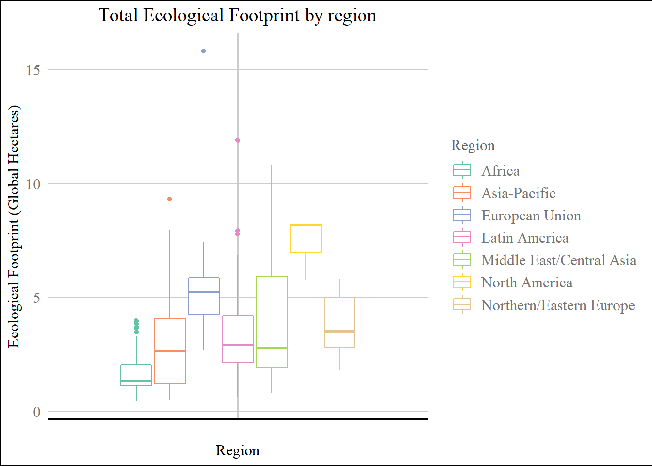

Total Biocapacity by Region

p3<- ggplot(footprint) +
  aes(x = "", y = Total.Biocapacity, colour = Region) +
  geom_boxplot(shape = "circle", fill = "#ffffff") +
  scale_color_brewer(palette = "Set2", direction = 1) +
  labs(
    x = "Region",
    y = "Biocapacity (Global Hectares)",
    title = "Total Biocapacity by region"
  ) +
  ggthemes::theme_gdocs() + theme(axis.title = element_text(family = "serif",
    colour = "black"), axis.text = element_text(family = "serif"),
    axis.text.x = element_text(family = "serif"),
    axis.text.y = element_text(family = "serif"),
    plot.title = element_text(family = "serif",
        size = 15, colour = "black", hjust = 0.5),
    legend.text = element_text(family = "serif"),
    legend.title = element_text(family = "serif"))

p3 + ylim(0,17)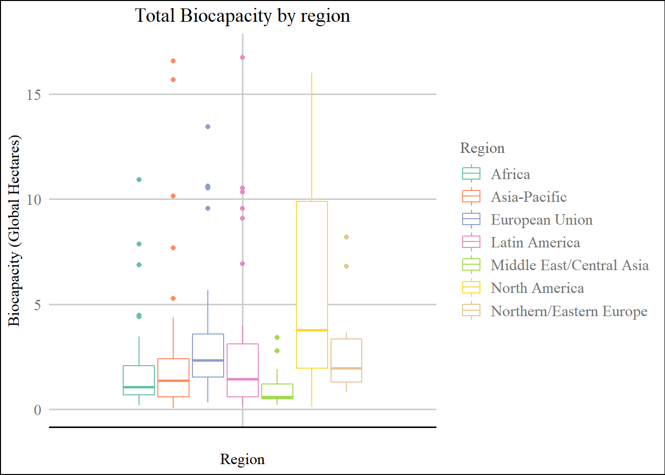

Data Exploration (Top 10 Analysis)

Here, we create a list with the top 10 countries for each variable (Ecological Footprint & Biocapacity) using the top_n function from the dplyr library. Using these lists, we can then plot simple bar charts to give us a deeper look into the countries at the outliers of our data, which have either extremely high Ecological Footprints or high Biocapacities.

From the resultant plot, we can see that most of the countries in the top 10 of Ecological Footprint data are developed nations - with only Qatar, Trinidad and Tobago and Oman being the lesser developed of the 10. This is corroborated by research by Galli et al. (2012) and other researchers who find out that the developed world has a few factors which lead to overuse of natural resources due to industrialization and a better ability at extracting resources more efficiently. Luxembourg and Qatar stand out as having higher Ecological Footprints than all the rest of the outliers. Luxembourg is one of the smallest nations in and has one of the smallest population sizes in Europe. Yet, the country’s carbon footprint on a per capita basis is significantly higher than that of any other European nation. A big contributor to Luxembourg’s catastrophic carbon emissions is the car ownership rate as well as energy consumption per capita, which are both the highest in Europe. Luxembourg does not have a lot of energy being consumed from renewable sources (2.1%), which adds to the negative carbon balance. This analysis is however controversial in academic circles, where certain researchers believe that there exists a discrepancy between the data reported by the GFN and the actual data in Luxembourg and other countries Hild et al. (2010).

Top 10 Ecological Footprint countries

top_10 <- top_n(footprint, n=10, Total.Ecological.Footprint) %>% 
  arrange(desc(Total.Ecological.Footprint))


ggplot(top_10,aes(x= reorder(Country, -Total.Ecological.Footprint), y=Total.Ecological.Footprint, fill = Total.Ecological.Footprint))+
  scale_fill_gradient(
    low = "#fd9aa6",
    high = "#FB0421",
    space = "Lab",
    na.value = "grey50",
    guide = "colourbar",
    aesthetics = "fill")+ 
  geom_col()+
  theme(axis.text.x = element_text(angle = 40, vjust = 1, hjust =1),
        legend.position = "none")+
  
  # Changing labels
  
  labs(y = "Total Ecological Footprint (Global Hectares)",
       x = '',
       title = "Highest Ecological Footprint Countries",
       caption = 'Source: Global Ecoogical Footprint, Global Footprint Network')+
    theme(plot.subtitle = element_text(family = "serif"),
    plot.caption = element_text(family = "serif"),
    panel.grid.major = element_line(colour = "gray94"),
    panel.grid.minor = element_line(colour = "white"),
    axis.title = element_text(family = "serif"),
    plot.title = element_text(family = "serif",
        size = 15, hjust = 0.5), legend.title = element_text(family = "serif"),
    panel.background = element_rect(fill = "white",
        colour = "white")) +labs(x = NULL) + theme(axis.text = element_text(family = "serif"),
    axis.text.x = element_text(family = "serif"),
    axis.text.y = element_text(family = "serif"),
    legend.text = element_text(family = "serif"))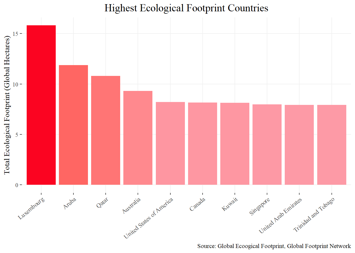

Top 10 Biocapacity countries

# Selecting top 10 countries and arranging by Biocapacity

top2_10 <- top_n(footprint, n=10, Total.Biocapacity) %>% 
  arrange(desc(Total.Biocapacity))

ggplot(top2_10,aes(x= reorder(Country, -Total.Biocapacity), y=Total.Biocapacity, fill = Total.Biocapacity))+
  scale_fill_gradient(
    low = "#9BC8AE",
    high = "#067736",
    space = "Lab",
    na.value = "grey50",
    guide = "colourbar",
    aesthetics = "fill")+ 
  geom_col()+
  theme(axis.text.x = element_text(angle = 40, vjust = 1, hjust =1),
        legend.position = "none")+
  
  # Changing labels
  
  labs(y = "Total Biocapacity (Global Hectares)",
       x = '',
       title = "Highest Biocapacity Countries",
       caption = 'Source: Global Ecoogical Footprint, Global Footprint Network')+
    theme(plot.subtitle = element_text(family = "serif"),
    plot.caption = element_text(family = "serif"),
    panel.grid.major = element_line(colour = "gray94"),
    panel.grid.minor = element_line(colour = "white"),
    axis.title = element_text(family = "serif"),
    plot.title = element_text(family = "serif",
        size = 15, hjust = 0.5), legend.title = element_text(family = "serif"),
    panel.background = element_rect(fill = "white",
        colour = "white")) +labs(x = NULL) + theme(axis.text = element_text(family = "serif"),
    axis.text.x = element_text(family = "serif"),
    axis.text.y = element_text(family = "serif"),
    legend.text = element_text(family = "serif"))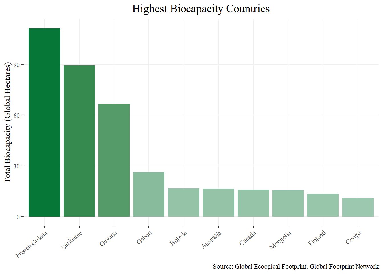

Relationship between HDI and Ecological Footprint/Biocapacity

In this section, we look at the various relationships that are connected to the main research question of this paper. Do HDI and GDP (socio-economic factors) have a relationship with Ecological Footprint or Biocapacity? While regression models will help with the inference for particular countries, the dataset limits us here to do a cross-sectional visualization. To add in more elements to the visualization, regionwise categories and the population size (in millions) was added to the scatter plot, giving us more dimensions to look at the data with.

This relationship is looked at by various scholars and researchers, where the complicated issue of ecological footprint versus human development is at the forefront. Kassouri and Altıntaş (2020) talk about the presence of a strong trade-off between the ecological footprint and human well-being captured by human development index. This is further corroborated by Ahmad et al. (2020), who concluded that economic growth and unrestricted usage of resources does lead to a growing ecological footprint. This brings back to the question regarding the Sustainable Development Goals, where countries vowed to progress with sustainability in mind. Is this really the case? Developed nations spearheaded this approach, and expected developing nations to follow their recommendations.

From the resultant plots in this section, we can see a increasing relationship when we look at HDI and ecological footprint. As HDI increases on the X-axis, we see a resultant increase to the Y-axis which shows the total Ecological Footprint of that corresponding nation. This has interesting implications as the difference between economic growth and development is fuzzy, and the HDI tries to look at a mixture of variables which indicate both of them. However, does this also mean that a growth in HDI would lead to better biocapacity in countries around the world?

This is proven to be incorrect as seen from the second plot, which looks at the relationship mentioned above. There is little evidence that all regions increase in their biocapacity as was the case with the ecological footprint. The implications for this is also interesting, where we see that increasing HDI does not

Relationship between HDI and Ecological Footprint

hdi1<-ggplot(footprint) +
 aes(x = HDI, y = Total.Ecological.Footprint, colour = Region, size = Population.millions) +
 geom_point(shape = "circle") +
 scale_color_brewer(palette = "Dark2", direction = 1) +
 labs(x = "HDI", 
 y = "Total Ecological Footprint (Global Hectares)", title = "Relationship between HDI and Ecological Footprint", 
 size = "Population (Millions)") +
 ggthemes::theme_gdocs()+ theme(plot.caption = element_text(family = "serif",
    hjust = 1.25), axis.title = element_text(family = "serif",
    colour = "black"), axis.text = element_text(family = "serif"),
    axis.text.x = element_text(family = "serif"),
    axis.text.y = element_text(family = "serif"),
    plot.title = element_text(family = "serif",
        size = 15, colour = "black", hjust = 0.5),
    legend.text = element_text(family = "serif"),
    legend.title = element_text(family = "serif")) +labs(caption = "Source: Global Footprint Network (GFN)")

hdi1 + geom_smooth(se=FALSE, method=lm)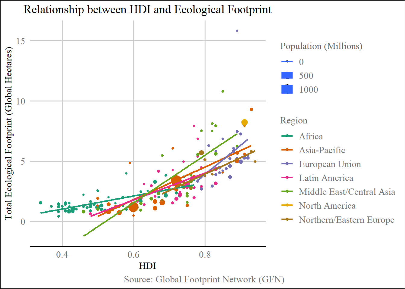

Relationship between HDI and Biocapacity

hdi2<-ggplot(footprint) +
  aes(x = HDI, y = Total.Biocapacity, colour = Region, size = Population.millions) +
  geom_point(shape = "circle") +
  scale_color_brewer(palette = "Dark2", direction = 1) +
  labs(x = "HDI", 
       y = "Total Biocapacity (Global Hectares)", title = "Relationship between HDI and Biocapacity", 
       size = "Population (Millions)") +
  ggthemes::theme_gdocs()+ theme(plot.caption = element_text(family = "serif",
                                                             hjust = 1.25), axis.title = element_text(family = "serif",
                                                                                                      colour = "black"), axis.text = element_text(family = "serif"),
                                 axis.text.x = element_text(family = "serif"),
                                 axis.text.y = element_text(family = "serif"),
                                 plot.title = element_text(family = "serif",
                                                           size = 15, colour = "black", hjust = 0.5),
                                 legend.text = element_text(family = "serif"),
                                 legend.title = element_text(family = "serif")) +labs(caption = "Source: Global Footprint Network (GFN)")

hdi2 + ylim(0,17) + geom_smooth(se=FALSE, method=lm)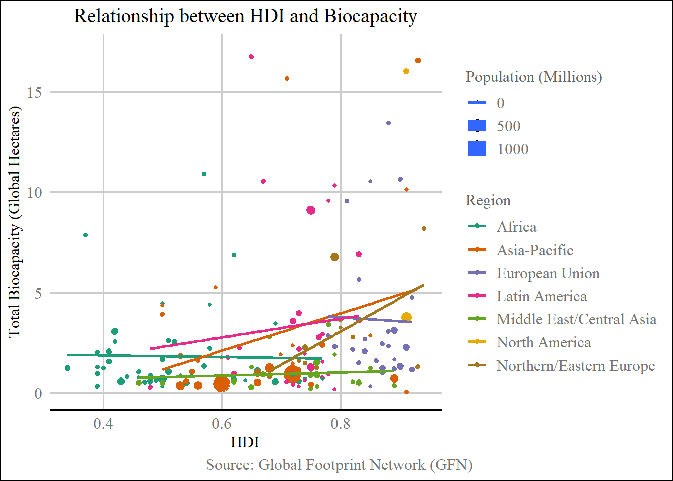

Relationship between GDP per Capita and Ecological Footprint/Biocapacity

In this section, the second part of the research question will be looked at. Do we see a connection between GDP per Capita, which is the operationalization for economic growth and income growth, with the Ecological Footprint or Biocapacity of nations? To further make the plot interactive, the package plotly is used, which gives us even more access to look at the graph in greater detail. Here, a new variable - the Ecological Deficit/Reserve, as was defined earlier in the paper. Here, we once again return back to our original hypothesis - increase in consumption leads to increased environmental impacts. This is the focus for many researchers who try to look at specific industries that negatively affect the environment, while at the same time not increasing the biocapacity. Kubiszewski et al. (2013) look at historical data on GDP and Ecological Footprint, where they surmise that efforts to increase the GDP has led to there being a deficit when looking at Ecological Footprint/Biocapacity. But as we move forward in the technological age where innovation is the primary commodity being sold between countries and sought after, will this remain the case?

Logic implies us to believe that efficiency increases will lead to a reversal in the plots that are attached below. We see that there is a positive correlation between GDP per Capita and Ecological Footprint, where countries such as Luxembourg, Qatar, etc. have a deficit. However, we can also see that Sweden and Australia have a Ecological reserve, while having a high GDP per Capita. Highly technological countries which have controlled for various other factors such as overpopulation, resource management, etc. do stand a chance to reverse the trends that we see here. In a paper by Szigeti, Toth, and Szabo (2017), the authors have collated time series data and run tests that empirically prove that there is a reversal happening. The authors mention efficiency gains due to a technology variable which was not significant in earlier years of the data.

GDP per Capita & Ecological Footprint

## data cleaning


footprint1 <- footprint %>%
  mutate(Country = as.character(Country), GDP.per.Capita = as.numeric(gsub("[$,]",
                                                                           "", footprint$GDP.per.Capita)), HDI = round(HDI,
                                                                                                                       2), Countries.Required = round(Countries.Required,
                                                                                                                                                      2), Biocapacity.Deficit = as.factor(ifelse(Biocapacity.Deficit >
                                                                                                                                                                                                   0, "Reserve", "Deficit"))) %>%
  rename(Status = Biocapacity.Deficit) %>%
  select(-c(Data.Quality)) %>%
  drop_na()


# Scatterplot between GDP and Ecological Footprint

scat_plot_data <- footprint1 %>%
  select(Country, Population.millions, GDP.per.Capita,
         HDI, Total.Ecological.Footprint, Status) %>%
  rename(Population.in.millions = Population.millions,
         Human.Development.Index = HDI, Ecological.Footprint = Total.Ecological.Footprint) %>%
  mutate(text = paste0("Country: ", Country, "<br>",
                       "HDI: ", Human.Development.Index, "<br>", "Ecological Footprint: ",
                       Ecological.Footprint, "<br>", "GDP per Capita: ",
                       "$", GDP.per.Capita))

scat_plot <- ggplot(scat_plot_data, aes(x = GDP.per.Capita,
                                        y = Ecological.Footprint, text = text)) + geom_smooth(col = "#61380B",
                                                                                              size = 0.7) + geom_point(aes(color = Status, size = GDP.per.Capita)) +
  scale_y_continuous(limits = c(0, 18)) + scale_color_manual(values = c("#DF0101",
                                                                        "#04B486")) + labs(title = "GDP on Ecological Footprint",
                                                                                           y = "Ecological Footprint", x = "GDP Per Capita") +
  theme(plot.title = element_text(face = "bold",
                                  size = 14, hjust = 0), panel.background = element_rect(fill = "#ffffff"),
        panel.grid.major.x = element_line(colour = "grey"),
        panel.grid.major.y = element_line(colour = "grey"),
        axis.line.x = element_line(color = "grey"),
        axis.line.y = element_line(color = "grey"),
        axis.text = element_text(size = 10, colour = "black"),
        legend.title = element_blank()) + theme(axis.title = element_text(family = "serif"),
    plot.title = element_text(family = "serif",
        size = 15, face = "plain", hjust = 0.5),
    legend.text = element_text(family = "serif"),
    legend.title = element_text(family = "serif"))

ggplotly(scat_plot, tooltip = "text") %>%
  layout(legend = list(orientation = "v", y = 1,
                       x = 0))

GDP per Capita & Biocapacity

scat_plot_data1 <- footprint1 %>%
  select(Country, Population.millions, GDP.per.Capita,
         HDI, Total.Biocapacity, Status) %>%
  rename(Population.in.millions = Population.millions,
         Human.Development.Index = HDI, Biocapacity = Total.Biocapacity) %>%
  mutate(text = paste0("Country: ", Country, "<br>",
                       "HDI: ", Human.Development.Index, "<br>", "Biocapacity: ",
                       Biocapacity, "<br>", "GDP per Capita: ",
                       "$", GDP.per.Capita))

scat_plot1 <- ggplot(scat_plot_data1, aes(x = GDP.per.Capita,
                                        y = Biocapacity, text = text)) + geom_smooth(col = "#61380B",
                                                                                              size = 0.7) + geom_point(aes(color = Status, size = GDP.per.Capita)) +
  scale_y_continuous(limits = c(0, 18)) + scale_color_manual(values = c("#DF0101",
                                                                        "#04B486")) + labs(title = "GDP on Biocapacity",
                                                                                           y = "Biocapacity", x = "GDP Per Capita") +
  theme(plot.title = element_text(face = "bold",
                                  size = 14, hjust = 0), panel.background = element_rect(fill = "#ffffff"),
        panel.grid.major.x = element_line(colour = "grey"),
        panel.grid.major.y = element_line(colour = "grey"),
        axis.line.x = element_line(color = "grey"),
        axis.line.y = element_line(color = "grey"),
        axis.text = element_text(size = 10, colour = "black"),
        legend.title = element_blank()) + theme(axis.title = element_text(family = "serif"),
    plot.title = element_text(family = "serif",
        size = 15, face = "plain", hjust = 0.5),
    legend.text = element_text(family = "serif"),
    legend.title = element_text(family = "serif"))

ggplotly(scat_plot1, tooltip = "text") %>%
  layout(legend = list(orientation = "v", y = 1,
                       x = 0))

References

Ahmad, Mahmood, Ping Jiang, Abdul Majeed, Muhammad Umar, Zeeshan Khan, and Sulaman Muhammad. 2020. “The Dynamic Impact of Natural Resources, Technological Innovations and Economic Growth on Ecological Footprint: An Advanced Panel Data Estimation.” Resources Policy 69: 101817.

Galli, Alessandro, Justin Kitzes, Valentina Niccolucci, Mathis Wackernagel, Yoshihiko Wada, and Nadia Marchettini. 2012. “Assessing the Global Environmental Consequences of Economic Growth Through the Ecological Footprint: A Focus on China and India.” Ecological Indicators 17: 99–107.

Hild, Paula, Bianca Schmitt, Antoine Decoville, Morgane Mey, and Joëlle Welfring. 2010. “Ecological Footprint of Luxembourg – Technical Report.” https://doi.org/10.13140/RG.2.2.10249.95844.

Kassouri, Yacouba, and Halil Altıntaş. 2020. “Human Well-Being Versus Ecological Footprint in MENA Countries: A Trade-Off?” Journal of Environmental Management 263: 110405.

Kubiszewski, Ida, Robert Costanza, Carol Franco, Philip Lawn, John Talberth, Tim Jackson, and Camille Aylmer. 2013. “Beyond GDP: Measuring and Achieving Global Genuine Progress.” Ecological Economics 93: 57–68.

Szigeti, Cecilia, Gergely Toth, and Daniel Robert Szabo. 2017. “Decoupling–Shifts in Ecological Footprint Intensity of Nations in the Last Decade.” Ecological Indicators 72: 111–17.

Toth, Gergely, and Cecı́lia Szigeti. 2016. “The Historical Ecological Footprint: From over-Population to over-Consumption.” Ecological Indicators 60: 283–91.

Posted on:: December 7, 2021

Length:: 31 minute read, 6506 words

See Also: